NORTON'S THEOREM

Click or Tap the Example circuits below to invoke TINACloud and select the Interactive DC mode to Analyze them Online.
Get a low cost access to TINACloud to edit the examples or create your own circuits

THÉVENIN’S THEOREM

MAXIMUM POWER TRANSFER THEOREM

Norton’s Theorem allows us to replace a complicated circuit with a simple equivalent circuit containing only a current source and a parallel connected resistor. This theorem is very important from both theoretical and practical viewpoints.

Concisely stated, Norton’s Theorem says:

Any two-terminal linear circuit can be replaced by an equivalent circuit consisting of a current source (I_N) and a parallel resistor (R_N).

It is important to note that the Norton equivalent circuit provides equivalence at the terminals only. Obviously, the internal structure and therefore the characteristics of the original circuit and its Norton equivalent are quite different.

Using Norton’s theorem is especially advantageous when:

We want to concentrate on a specific portion of a circuit. The rest of the circuit can be replaced by a simple Norton equivalent.

We have to study the circuit with different load values at the terminals. Using the Norton equivalent, we can avoid having to analyze the complex original circuit each time.

We can calculate the Norton equivalent in two steps:

Calculate R_N. Set all sources to zero (replace voltage sources by short circuits and current sources by open circuits) and then find the total resistance between the two terminals.

Calculate I_N.Find the short circuit current between the terminals. It is the same current that would be measured by an ammeter placed between the terminals.

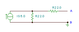
To illustrate, let’s find Norton’s equivalent circuit for the circuit below.

Click/tap the circuit above to analyze on-line or click this link to Save under Windows

The TINA solution illustrates the steps needed for the calculation of the Norton parameters :

Of course, the parameters can be easily calculated by the rules of series-parallel circuits described in previous chapters:

R_N = R₂ + R₂ = 4 ohm.

The short-circuit current (after restoring the source!) can be calculated using current division:

The resulting Norton equivalent circuit:

{Solution by TINA’s Interpreter}
{The resistance of the killed network}
RN:=R2+R2;
{The Norton’s source current is the
short circuited current in the branch of R1}
IN:=Is*R2/(R2+R2);
IN=[2.5]
RN=[4]
{Finally the asked current}
I:=IN*RN/(RN+R1);
I=[2]
{Using current division}
Id:=Is*R2/(R2+R2+R1);
Id=[2]

#Solution by Python!
#The resistance of the killed network:
RN=R2+R2
#The Norton’s source current is the
#short circuited current in the branch of R1:
IN=Is*R2/(R2+R2)
print(“IN= %.3f”%IN)
print(“RN= %.3f”%RN)
#Finally the asked current:
I=IN*RN/(RN+R1)
print(“I= %.3f”%I)
#Using current division:
Id=Is*R2/(R2+R2+R1)
print(“Id= %.3f”%Id)

Further examples:

Example 1

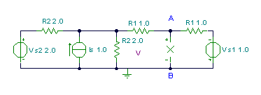
Find the Norton equivalent for the AB terminals of the circuit below

Click/tap the circuit above to analyze on-line or click this link to Save under Windows

Find the current of the Norton equivalent using TINA by connecting a short circuit to the terminals, and then the equivalent resistance by disabling the generators.

Surprisingly, you can see that the Norton source might be zero current.

Therefore, the resulting Norton equivalent of the network is just a 0.75 Ohm resistor.

{Solution by TINA’s Interpreter!}
{Use mesh current method!}
sys Isc,I1,I2
-Vs2+I1*(R2+R2)+Is*R2-Isc*R2+I2*R2=0
Isc*(R1+R2)-Is*R2-I1*R2-I2*(R1+R2)=0
I2*(R1+R1+R2)-Isc*(R1+R2)+Is*R2+I1*R2+Vs1=0
end;
Isc=[0]
Req:=Replus(R1,(R1+Replus(R2,R2)));
Req=[666.6667m]

#Solution by Python!
import numpy as np
# Ax=b

#Define replus using lambda:
Replus= lambda R1, R2 : R1*R2/(R1+R2)

#Write up the matrix
#of the coefficients:
A = np.array(
[[R2+R2, R2, -R2],
[-R2, -(R1+R2), R1+R2],
[R2, R1+R1+R2, – (R1+R2)]])

#Write up the matrix
#of the constants:
b = np.array([Vs2-Is*R2, Is*R2, -Is*R2-Vs1])

x = np.linalg.solve(A, b)
I1=x[0]
I2=x[1]
Isc=x[2]
print(“Isc= %.3f”%Isc)
Req=Replus(R1,R1+Replus(R2,R2))
print(“Req= %.3f”%Req)

Example 2

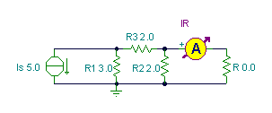
This example shows how the Norton equivalent simplifies calculations.

Find the current in the resistor R if its resistance is:

1.) 0 ohm; 2.) 1.8 ohm; 3.) 3.8 ohm 4.) 1.43 ohm

Click/tap the circuit above to analyze on-line or click this link to Save under Windows

First, find the Norton equivalent of the circuit for the terminal pair connected to R by substituting for R an open circuit.

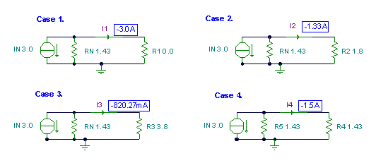
Finally, use the Norton equivalent to calculate the currents for the different loads:

{Solution by TINA’s Interpreter}
Ri1:=0;
Ir1:=-Is*R1/(R1+R3+replus(R2,Ri1))*R2/(R2+Ri1);
Ri2:=1.8;
Ir2:=-Is*R1/(R1+R3+replus(R2,Ri2))*R2/(R2+Ri2);
Ri3:=3.8;
Ir3:=-Is*R1/(R1+R3+replus(R2,Ri3))*R2/(R2+Ri3);
Ri4:=1.42857;
Ir4:=-Is*R1/(R1+R3+replus(R2,Ri4))*R2/(R2+Ri4);
Ir1=[-3]
Ir2=[-1.3274]
Ir3=[-819.6721m]
Ir4=[-1.5]

#Solution by Python!
#First define replus using lambda:
replus= lambda R1, R2 : R1*R2/(R1+R2)
Ri1=0
Ir1=-Is*R1/(R1+R3+replus(R2,Ri1))*R2/(R2+Ri1)
Ri2=1.8
Ir2=-Is*R1/(R1+R3+replus(R2,Ri2))*R2/(R2+Ri2)
Ri3=3.8
Ir3=-Is*R1/(R1+R3+replus(R2,Ri3))*R2/(R2+Ri3)
Ri4=1.42857
Ir4=-Is*R1/(R1+R3+replus(R2,Ri4))*R2/(R2+Ri4)
print(“Ir1= %.3f”%Ir1)
print(“Ir2= %.3f”%Ir2)
print(“Ir3= %.3f”%Ir3)
print(“Ir4= %.3f”%Ir4)

THÉVENIN’S THEOREM

MAXIMUM POWER TRANSFER THEOREM