 Click or Tap the Example circuits below to invoke TINACloud and select the Interactive DC mode to Analyze them Online.
 Get a low cost access to TINACloud to edit the examples or create your own circuits
We have already seen that an AC circuit can (at one frequency) be replaced by a Thévenin or Norton equivalent circuit. Based on this technique, and with the Maximum Power Transfer Theorem for DC circuits, we can determine the conditions for an AC load to absorb maximum power in an AC circuit. For an AC circuit, both the Thévenin impedance and the load can have a reactive component. Although these reactances do not absorb any average power, they will limit the circuit current unless the load reactance cancels the reactance of the Thévenin impedance. Consequently, for maximum power transfer, the Thévenin and load reactances must be equal in magnitude but opposite in sign; furthermore, the resistive parts -according to the DC maximum power theorem- must be equal. In another words the load impedance must be the conjugate of the equivalent Thévenin impedance. The same rule applies for the load and Norton admittances.
RL= Re{ZTh} and XL = – Im{ZTh}
The maximum power in this case:
Pmax = 
Where V2Th and I2N represent the square of the sinusoidal peak values.
We’ll next illustrate the theorem with some examples.
Example 1
R1 = 5 kohm, L = 2 H, vS(t) = 100V cos wt, w = 1 krad/s.
a) Find C and R2 so that the average power of the R2-C two-pole will be maximum
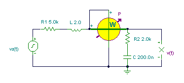
b) Find the maximum average power and the reactive power in this case.
c) Find v(t) in this case.
The solution by the theorem using V, mA, mW, kohm, mS, krad/s, ms, H, m F units:v
a.) The network is already in Thévenin form, so we can use the conjugate form and determine the real and imaginary components of ZTh:
R2 = R1 = 5 kohm; wL = 1/w C = 2 ® C = 1/w2L = 0.5 mF = 500 nF.
b.) The average power:
Pmax = V2/(4*R1) = 1002/(2*4*5) = 250 mW
The reactive power: first the current:
I = V / (R1 + R2 + j(wL – 1/wC)) = 100/10 = 10 mA
Q = – I2/2 * XC = – 50*2 = – 100 mvarc.) The load voltage in the case of maximum power transfer:
VL = I*(R2 + 1/ (j w C ) = 10*(5-j/(1*0.5)) =50 – j 20 = 53.852 e -j 21.8° V
and the time function: v(t) = 53.853 cos (wt – 21.8°) V
V:=100;
om:=1000;
{a./} R2b:=R1;
C2:=1/sqr(om)/L;
C2=[500n]
{b./} I2:=V/(R1+R2b);
P2m:=sqr(abs(I2))*R2b/2;
Q2m:=-sqr(abs(I2))/om/C2/2;
P2m=[250m]
Q2m=[-100m]
{c./} V2:=V*(R2b+1/j/om/C2)/(R1+R2b);
abs(V2)=[53.8516]
import cmath as c
#Lets simplify the print of complex
#numbers for greater transparency:
cp= lambda Z : “{:.8f}”.format(Z)
V=100
om=1000
#a./
R2b=R1
C2=1/om**2/L
print(“C2=”,cp(C2))
#b./
I2=V/(R1+R2b)
P2m=abs(I2)**2*R2b/2
Q2m=-abs(I2)**2/om/C2/2
print(“P2m=”,cp(P2m))
print(“Q2m=”,cp(Q2m))
#c./
V2=V*(R2b+1/1j/om/C2)/(R1+R2b)
print(“abs(V2)=”,cp(abs(V2)))
Example 2
vS(t) = 1V cos w t, f = 50 Hz,
R1 = 100 ohm, R2 = 200 ohm, R = 250 ohm, C = 40 uF, L = 0.5 H.
a.) Find the power in the load R-L
b.) Find R and L so that the average power of the R-L two-pole will be maximum.

First we have to find the Thévenin generator which we will substitute for the circuit to the left of the nodes of the R-L load.
The steps:
1. Remove the load R-L and substitute an open circuit for it
2. Measure (or compute) the open circuit voltage
3. Replace the voltage source with a short circuit (or replace the current sources by open circuits)
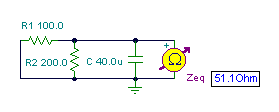
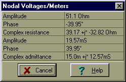
4. Find the equivalent impedance

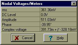

Use V, mA, kohm, krad/s, mF, H, ms units!




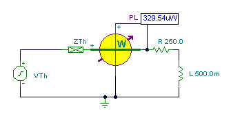
And finally the simplified circuit:
Solution for power: I = VTh /(ZTh + R + j w L) = 0.511/ (39.17 + 250 – j 32.82 + j 314*0.5)
½I½=1.62 mA and P = ½I½2 * R/2 = 0.329 mWWe find the maximum power if

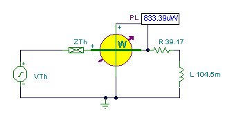
The maximum power:
Imax = 0.511/(2*39.17) = 6.52 mA and 
Vs:=1;
om:=100*pi;
va:=Vs*replus(replus(R2,(1/j/om/C)),(R+j*om*L))/(R1+replus(replus(R2,(1/j/om/C)),(R+j*om*L)));
abs(va)=[479.3901m]
PR:=sqr(abs(va/(R+j*om*L)))*R/2;
QL:=sqr(abs(va/(R+j*om*L)))*om*L/2;
PR=[329.5346u]
QL=[207.0527u]
{b./} Zb:=(replus(replus(R1,R2),1/j/om/C));
abs(Zb)=[51.1034]
VT:=Vs*replus(R2,1/j/om/C)/(R1+replus(R2,1/j/om/C));
VT=[391.7332m-328.1776m*j]
abs(VT)=[511.0337m]
R2b:=Re(Zb);
Lb:=-Im(Zb)/om;
Lb=[104.4622m]
R2b=[39.1733]
import cmath as c
#Lets simplify the print of complex
#numbers for greater transparency:
cp= lambda Z : “{:.8f}”.format(Z)
#Define replus using lambda:
Replus= lambda R1, R2 : R1*R2/(R1+R2)
Vs=1
om=100*c.pi
va=Vs*Replus(Replus(R2,1/1j/om/C),R+1j*om*L)/(R1+Replus(Replus(R2,1/1j/om/C),R+1j*om*L))
print(“abs(va)=”,cp(abs(va)))
PR=abs(va/(R+1j*om*L))**2*R/2
QL=abs(va/(R+1j*om*L))**2*om*L/2
print(“PR=”,cp(PR))
print(“QL=”,cp(QL))
#b./
Zb=Replus(Replus(R1,R2),1/1j/om/C)
print(“abs(Zb)=”,abs(Zb))
VT=Vs*Replus(R2,1/1j/om/C)/(R1+Replus(R2,1/1j/om/C))
print(“VT=”,cp(VT))
print(“abs(VT)=”,cp(abs(VT)))
R2b=Zb.real
Lb=-Zb.imag/om
print(“Lb=”,cp(Lb))
print(“R2b=”,cp(R2b))
Here we used TINA’s special function replus to find the parallel equivalent of two impedances.