 Click or Tap the Example circuits below to invoke TINACloud and select the Interactive DC mode to Analyze them Online.
 Get a low cost access to TINACloud to edit the examples or create your own circuits
Another way of simplifying the complete set of Kirchhoff’s equations is the mesh or loop current method. Using this method, Kirchhoff’s current law is satisfied automatically, and the loop equations that we write also satisfy Kirchhoff’s voltage law. Satisfying Kirchhoff’s current law is achieved by assigning closed current loops called mesh or loop currents to each independent loop of the circuit and using these currents to express all the other quantities of the circuit. Since the loop currents are closed, the current that flows into a node must also flow out of the node; so writing node equations with these currents leads to identity.
Let us first consider the method of mesh currents.
We first note that the mesh current method is only applicable for “planar” circuits. Planar circuits have no crossing wires when drawn on a plane. Often, by redrawing a circuit which appears to be non-planar, you can determine that it is, in fact, planar. For non-planar circuits, use the loop current method described later in this chapter.
To explain the idea of mesh currents, imagine the branches of the circuit as “fishing net” and assign a mesh current to each mesh of the net. (Sometimes it is also said that a closed current loop is assigned in each “window” of the circuit.)
    |
The technique of representing the circuit by a simple drawing, called a graph, is quite powerful. Since Kirchhoff’s laws do not depend on the nature of the components, you can disregard the concrete components and substitute for them simple line segments, called the branches of the graph. Representing circuits by graphs allows us to use the techniques of mathematical graph theory. This helps us explore the topological nature of a circuit and determine the independent loops. Come back later to this site to read more about this topic.
The steps of mesh current analysis:
Assign a mesh current to each mesh. Although the direction is arbitrary, it is customary to use the clockwise direction.
Apply Kirchhoff’s voltage law (KVL) around each mesh, in the same direction as the mesh currents. If a resistor has two or more mesh currents through it, the total current through the resistor is calculated as the algebraic sum of the mesh currents. In other words, if a current flowing through the resistor has the same direction as the mesh current of the loop, it has a positive sign, otherwise a negative sign in the sum. Voltage sources are taken into account as usual, If their direction is the same as the mesh current, their voltage is taken to be positive, otherwise negative, in the KVL equations. Usually, for current sources, only one mesh current flows through the source, and that current has the same direction as the current of the source. If this is not the case, use the more general loop current method, described later in this paragraph. There is no need to write KVL equations for loops containing mesh currents assigned to current sources.
Solve the resulting loop equations for the mesh currents.
Determine any requested current or voltage in the circuit using the mesh currents.
Let us illustrate the method by the following example:
Find the current I in the circuit below.
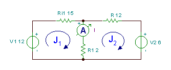
We see that there are two meshes (or a left and right window) in this circuit. Let’s assign the clockwise mesh currents J1 and J2 to the meshes. Then we write the KVL equations, expressing the voltages across the resistors by Ohm’s law:
-V1 + J1*(Ri1+R1) – J2*R1 = 0
V2 – J1*R1 + J2*(R + R1) = 0
Numerically:
-12 + J1*17 – J2*2 = 0
6 – J1*2 +J2*14 = 0
Express J1 from the first equation: J1 = 

multiply by 17: 102 – 24 + 4*J2 + 238*J2 = 0 hence J2 = 
and J1 = 
Finally, the required current:

{Mesh current method}
Sys J1,J2
J1*(Ri1+R1)-J2*R1-V1=0
J1*R1+J2*(R1+R)+V2=0
end;
J1=[666.6667m]
J2=[-333.3333m]
I:=J1-J2;
I=[1]
import numpy as n
#Use mesh current method!
#We have a linear system of equations that we want to solve
#for I1,I2:
#I1*(Ri1+R1)+I2*Ri1-V1=0
#-V1+I1*Ri1+I2*(Ri1+R)+V2=0
#Write up the matrix of the coefficients:
A=n.array([[Ri1+R1,Ri1],[Ri1,Ri1+R]])
#Write up the matrix of the constants:
b=n.array([V1,V1-V2])
x=n.linalg.solve(A,b)
I1=x[0]
I2=x[1]
print(“I1= %.3f”%I1)
print(“I2= %.3f”%I2)
I=I1
print(“I= %.3f”%I)
Let’s check the results with TINA:
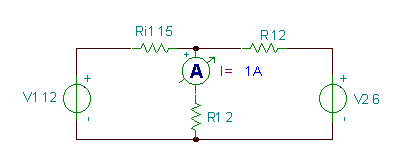

Next, let’s solve the previous example again, but with the more general method of loop currents. Using this method, the closed current loops, called loop currents, are assigned not necessarily to the meshes of the circuit, but to arbitrary independent loops. You can ensure that the loops are independent by having at least one component in each loop that is not contained in any other loop. For planar circuits, the number of the independent loops is the same as the number of meshes, which is easy to see.
A more precise way of determining the number of independent loops is as follows.
Given a circuit with b branches and N nodes. The number of the independent loops l is:
l = b – N + 1
This follows from fact that the number of independent Kirchhoff’s equations must be equal to the branches in the circuit, and we already know that there are only N-1 independent node equations. Therefore the total number of the Kirchhoff’s equations is
b = N-1 + l and hence l = b – N + 1
This equation also follows from the fundamental theorem of graph theory which will be described later at this site.
Now let’s solve the previous example again, but more simply, by using the loop current method. With this method we are free to use loops in meshes or any other loops, but let’s keep the loop with J1 in the left mesh of the circuit. However, for the second loop we choose the loop with J2, as shown in the figure below. The advantage of this choice is that J1 will be equal to the requested current I, since it is the only loop current passing through R1. This means that we don’t need to calculate J2 at all. Note that, unlike “real” currents, the physical meaning of loop currents is dependent upon how we assign them to the circuit.
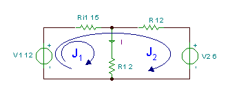

The KVL equations:
J1*(R1+Ri1) + J2*R i1 – V1 = 0
-V1+J1*Ri1+J2*(R + Ri) + V2 = 0
and the required current: I = J1
Numerically: J1*(15+2)+J2*15-12 = 0
-12 + J1*15 + J2*(15+12) + 6 = 0
Express J2 from the second equation:

Substitute into the first equation:


Hence: J1 = I = 1 A
Further examples.
Example 1
Find the current I in the circuit below.
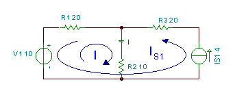
In this circuit, we use the method of loop currents. In the left window of the circuit we take a loop current which we denote with I since it is equal to the requested current. The other loop current is equal to the Is1 source current, so we denote it directly as IS1.
Note that that the direction of this loop current is not clockwise since its direction is determined by the current source. However, since this loop current is already known, there is no need to write the KVL equation for the loop where IS1 is taken.
Therefore the only equation to solve is:
-V1 + I*R2 + R1 *(I – IS1) = 0
hence
I= (V1 + R1 *IS1)/( R1 + R2)
Numerically
I=(10+20*4)/(20+10)=3 A
You can also generate this result calling TINA’s symbolic analysis from the Analysis/Symbolic Analysis/DC Result menu:
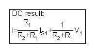
Or you can solve the KVL equation by the interpreter:
| {Solution by TINA’s Interpreter} {Use mesh current method} Sys I -V1 + I*R2 + R1 *(I – IS1) = 0 end; I=[3] |
The following example has 3 current sources and is very easy to solve by the method of loop currents.
Example 2
Find the voltage V.


In this example, we can choose three loop currents so that each passes through only one current source. Therefore, all the three loop currents are known, and we only need to express the unknown voltage, V, using them.
Making the algebraic sum of the currents through R3:
V= (IS3 – IS2)*R3=(10-5)*30 = 150 V. You can verify this with TINA:.


Next, let’s tackle again a problem that we have already solved in the Kirchhoff’s laws and Node potential method chapters.
Example 3
Find the voltage V of the resistor R4.
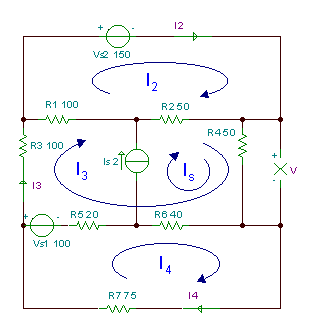

R1 = R3 = 100 ohm, R2 = R4 = 50 ohm, R5 = 20 ohm,R6 = 40 ohm, R7 = 75 ohm.
This problem needed at least 4 equations to solve in the previous chapters.
Solving this problem with the method of loop currents, we have four independent loops, but with the proper choice of loop currents, one of the loop currents will be equal to the source current Is.
Based on the loop currents shown in the figure above, the loop equations are:
VS1+I4*(R5+R6+R7) – IS*R6 –I3*(R5 + R6) = 0
VS2 – I3*(R1+R2) – IS*R2 + I2*(R1 + R2)= 0
-VS1 + I3*(R1 + R2 + R3 + R4 + R5 + R6) + IS*(R2 +R4 + R6) – I4*(R5 + R6) – I2*(R1 + R2) = 0
The unknown voltage V can be expressed by the loop currents:
V = R4 * (I2 + I3)
Numerically:
100+I4*135-2*40-I3*60 = 0
150+I2*150-2*50-I3*150 = 0
–100+I3*360+2*140-I4*60-I2*150 = 0
V = 50*(2+I3)
We can use Cramer’s rule to solve this system of equations:
I4 = D3/D
where D is the determinant of the system. D4, the determinant for I4, is formed by substituting the right hand side of the system is placed for the column of I4’s coefficients.
The system of equations in ordered form:
– 60* I3 +135*I4= -20
150*I2-150*I3 = – 50
-150*I2+360*I3 – 60*I4= – 180
So the determinant D:


The solution of this system of equations is:
V = R4*(2+I3) = 34.8485 V
You can confirm the answer via the result calculated by TINA.
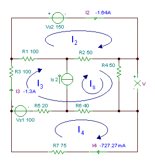
Sys I2,I3,I4
Vs2+I2*(R1+R2)-R2*Is-I3*(R1+R2)=0
-Vs1+I3*(R1+R2+R3+R4+R5+R6)+Is*(R2+R4+R6)-I2*(R1+R2)-I4*(R5+R6)=0
Vs1+I4*(R5+R6+R7)-Is*R6-I3*(R5+R6)=0
end;
I2=[-1.6364]
I3=[-1.303]
I4=[-727.2727m]
V:=R4*(Is+I3);
V=[34.8485]
import numpy as n
#We have a linear system of equations that we want to solve
#for I1,I2,I3,I4:
#I1=Is
#Vs2+I2*(R1+R2)-R2*I1-I3*(R1+R2)=0
#-Vs1+I3*(R1+R2+R3+R4+R5+R6)+I1*(R2+R4+R6)-I2*(R1+R2)-I4*(R5+R6)=0
#Vs1+I4*(R5+R6+R7)-I1*R6-I3*(R5+R6)=0
#Write up the matrix of the coefficients:
A=n.array([[1,0,0,0],[-R2,R1+R2,-(R1+R2),0],[R2+R4+R6,-(R1+R2),R1+R2+R3+R4+R5+R6,-(R5+R6)],[-R6,0,-(R5+R6),R5+R6+R7]])
#Write up the matrix of the constants:
b=n.array([Is,-Vs2,Vs1,-Vs1])
x=n.linalg.solve(A,b)
I1,I2,I3,I4=x[0],x[1],x[2],x[3]
print(“I1= %.5f”%I1) #x[0]=I1
print(“I2= %.5f”%I2) #x[1]=I2
print(“I3= %.5f”%I3) #x[2]=I1
print(“I4= %.5f”%I4) #x[3]=I2
V=R4*(I1+I3)
print(“V= %.5f”%V)
In this example, each unknown loop current is a branch current (I1, I3 and I4); so it is easy to check the result by comparison with the DC analysis results of TINA.
