 Click or Tap the Example circuits below to invoke TINACloud and select the Interactive DC mode to Analyze them Online.
 Get a low cost access to TINACloud to edit the examples or create your own circuits
The complete set of Kirchhoff’s equations can be significantly simplified by the node potential methoddescribed in this chapter. Using this method, Kirchhoff’s voltage law is satisfied automatically, and we need only write node equations to satisfyKirchhoff’s current law, too. Satisfying Kirchhoff’s voltage law is achieved by using node potentials (also called node or nodal voltages)with respect to a particular node called the reference node. In other words, all the voltages in the circuit are relative to the reference node, which is normally considered to have 0 potential. It is easy to see that with these voltage definitions Kirchhoff’s voltage law is satisfied automatically, since writing loop equations with these potentials leads to identity. Note that for a circuit having N nodes you should write only N – 1 equations. Normally, the node equation for the reference node is left out.
The sum of all currents in the circuit is zero since each current is flowing in and out of a node. Therefore, the Nth node equation is not independent from the previous N-1 equations. If we included all the N equations, we would have an unsolvable system of equations.
The node potential method (also called nodal analysis) is the method best suited to computer applications. Most circuit analysis programs–including TINA–are based on this method.
The steps of the nodal analysis:1. Pick a reference node with 0 node potential and label each remaining node with V1, V2 or j1, j2and so on.2. Apply Kirchhoff’s current law at each node except the reference node. Use Ohm’s law to express unknown currents from node potentials and voltage source voltages when necessary. For all unknown currents, assume the same reference direction (e.g. pointing out of the node) for each application of Kirchhoff’s current law.
3. Solve the resulting node equations for the node voltages.
4. Determine any requested current or voltage in the circuit using the node voltages.
Let us illustrate step 2 by writing the node equation for node V1 of the following circuit fragment:
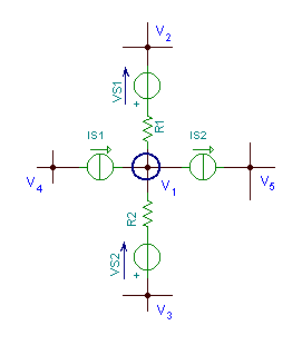

First, find the current from node V1 to node V2. We will use Ohm’s Law at R1. The voltage across R1 is V1 – V2 – VS1
And the current through R1 (and from node V1 to node V2) is


Note that this current has a reference direction pointing out of the V1 node. Using the convention for currents pointing out of a node, it should be taken into account in the node equation with a positive sign.
The current expression of the branch between V1 and V3 will be similar, but since VS2 is in the opposite direction from VS1 (which means the potential of the node between VS2 and R2 is V3-VS2), the current is


Finally, because of the indicated reference direction, IS2 should have a positive sign and IS1 a negative sign in the node equation.
The node equation:

Now let’s see a complete example to demonstrate the use of the node potential method.
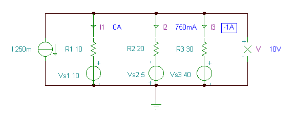
Find the voltage V and the currents through the resistors in the circuit below
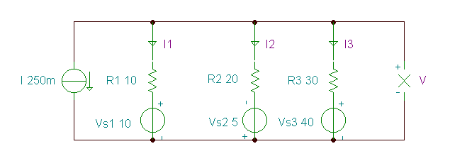
Since we have only two nodes in this circuit, we can reduce the solution to the determination of one unknown quantity.By choosing the lower node as a reference node, the unknown node voltage is the voltage we’re solving for, V.
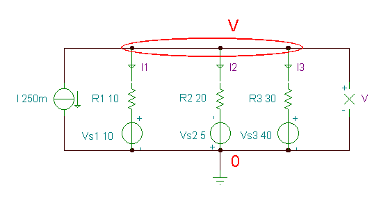
The nodal equation for the upper node:

Numerically:

Multiply by 30: 7.5+3V – 30 + 1.5 V + 7.5.+ V – 40 = 0 5.5 V –55 = 0
Hence: V = 10 V
Sys V
I+(V-Vs1)/R1+(V+Vs2)/R2+(V-Vs3)/R3=0
end;
V=[10]
import numpy as n, sympy as s
#I+(V-Vs1)/R1+(V+Vs2)/R2+(V-Vs3)/R3=0
#Write up the matrix of the coefficients:
A=n.array([[1/R1+1/R2+1/R3]])
#Write up the matrix of the constants:
b=n.array([-I+Vs1/R1-Vs2/R2+Vs3/R3])
V= n.linalg.solve(A,b)[0]
print(“%.3f”%V)
#Symbolic solution with sympy solve
V= s.symbols(‘V’)
sol = s.solve([I+(V-Vs1)/R1+(V+Vs2)/R2+(V-Vs3)/R3],[V])
print(sol)
Now let’s determine the currents through the resistors. This is easy, since the same currents are used in the nodal equation above.


{Use node potential method !}
Sys V
I+(V-Vs1)/R1+(V+Vs2)/R2+(V-Vs3)/R3=0
end;
V=[10]
{The currents of the resistors}
IR1:=(V-Vs1)/R1;
IR2:=(V+Vs2)/R2;
IR3:=(V-Vs3)/R3;
IR1=[0]
IR2=[750.0001m]
IR3=[-1000m]
We can check the result with TINA by simply turning on TINA’s DC interactive mode or using the Analysis / DC Analysis / Nodal Voltages command.
Next, let’s solve the problem which was already used as the last example of the Kirchhoff’s laws chapter
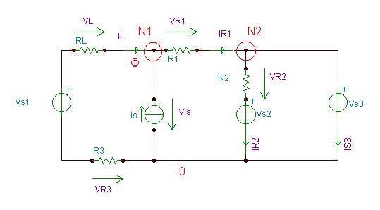
Find the voltages and currents of each element of the circuit.
Choosing the lower node as a reference node of 0 potential, the nodal voltage of N2 will be equal to VS3, : j2 = therefore we have only one unknown nodal voltage. You may remember that previously, using the full set of Kirchhoff’s equations, even after some simplifications, we had a linear system of equations of 4 unknowns.
Writing the node equations for node N1, let us denote the nodal voltage of N1 by j1
The simple equation to solve is:


Numerically:

Multiply by 330, we get:
3j1-360 – 660 + 11j1 – 2970 = 0 ® j1= 285 V
After calculating j1, it is easy to calculate the other quantities in the circuit.
The currents:


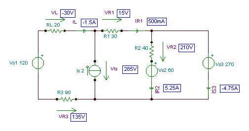
IS3 = IR1 – IR2 = 0.5 – 5.25 = – 4.75 A
And the voltages:
VIs = j1 = 285 V
VR1= (j1 – VS3) = 285 – 270 = 15 V
VR2 = (VS3 – VS2) = 270 – 60 =210 V


VL = -(j1-VS1-VR3) = -285 +120 +135 = – 30 V
You may note that with the node potential method you still need some extra calculation to determine the currents and voltages of the circuit. However these calculations are very simple, much simpler than solving linear equations systems for all circuit quantities simultaneously.
We can check the result with TINA by simply turning on TINA’s DC interactive mode or using Analysis / DC Analysis / Nodal Voltages command.
  |
Let’s see further examples.
Example 1
Find the current I.
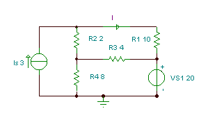
In this circuit there are four nodes, but since we have an ideal voltage source that determines the node voltage at its positive pole, we should chose its negative pole as the reference node. Therefore, we really have only two unknown node potentials: j1 and j2 .
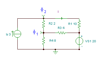
The equations for the nodes of potentials j1 and j2:


Numerically:


To solve this, multiply the first equation by 3 and the second by 2, then add the two equations:
11j1 =220
and hence j1= 20V, j2 = (50 + 5j1) / 6= 25 V
Finally the unknown current:

The solution of a system of linear equations can be also calculated using Cramer’s rule.
Let’s illustrate the use of Cramer’s rule by solving the system above again..
1. Fill in the matrix of the coefficients of unknowns:


Hence j1 = 20 V and j2 = 25 V
To check the result with TINA, simply turn on TINA’s DC interactive mode or use Analysis / DC Analysis / Nodal Voltages command. Note that using the Voltage Pin component of TINA, you can directly show the node potentials assuming that the Ground component is connected to the reference node.
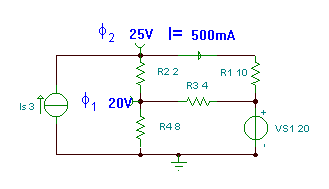
Sys fi1,fi2
(fi1-fi2)/R2+(fi1-VS1)/R3+fi1/R4=0
(fi2-fi1)/R2+(fi2-VS1)/R1-Is=0
end;
fi1=[20]
fi2=[25]
I:=(fi2-VS1)/R1;
I=[500m]
import numpy as n
#We have a system of
#llinear equations that
#we want to solve for fi1, fi2:
#(fi1-fi2)/R2+(fi1-VS1)/R3+fi1/R4=0
#(fi2-fi1)/R2+(fi2-VS1)/R1-Is=0
#Write up the matrix of the coefficients:
A=n.array([[1/R2+1/R3+1/R4,-1/R2],[-1/R2,1/R2+1/R1]])
#Write up the matrix of the constants:
b=n.array([[VS1/R3],[VS1/R1+Is]])
x=n.linalg.solve(A,b)
fi1,fi2=x[0],x[1]
print(“fi1= %.3f”%fi1)
print(“fi2= %.3f”%fi2)
I=(fi2-VS1)/R1
print(“I= %.3f”%I)
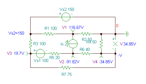
Example 2.
Find the voltage of the resistor R4.
R1 = R3 = 100 ohm, R2 = R4 = 50 ohm, R5 = 20 ohm, R6 = 40 ohm, R7 = 75 ohm
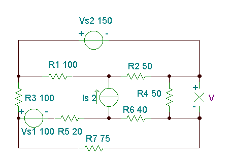
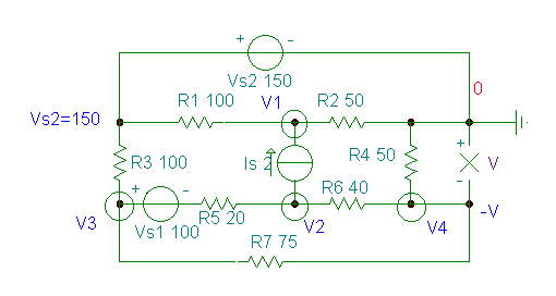
In this case, it is practical to choose the negative pole of the voltage source VS2 as the reference node because then the positive pole of the VS2 voltage source will have VS2 = 150 node potential. Because of this choice, however, the required V voltage is opposite to the node voltage of the node N4; therefore V4 = – V.
The equations:


We do not present the hand calculations here, since the equations can be easily solved by TINA’s interpreter.
{Use node potential method !}
Sys V,V1,V2,V3
V1/R2+(V1-Vs2)/R1-Is=0
(V2+V)/R6+(V2-V3+Vs1)/R5+Is=0
(V3+V)/R7+(V3-Vs2)/R3+(V3-Vs1-V2)/R5=0
(-V-V2)/R6-V/R4+(-V-V3)/R7=0
end;
V1=[116.6667]
V2=[-91.8182]
V3=[19.697]
V=[34.8485]
import numpy as n
#Use node potential method !
#We have a system of linear equations that we want to solve
#for V,V1,V2,V3:
#V1/R2+(V1-Vs2)/R1-Is=0
#(V2+V)/R6+(V2-V3+Vs1)/R5+Is=0
#(V3+V)/R7+(V3-Vs2)/R3+(V3-Vs1-V2)/R5=0
#(-V-V2)/R6-V/R4+(-V-V3)/R7=0
#Write up the matrix of the coefficients:
A= n.array([[0,1/R2+1/R1,0,0],[1/R6,0,1/R6+1/R5,(-1)/R5],[1/R7,0,(-1)/R5,1/R7+1/R5+1/R3],[(-1)/R6-1/R4-1/R7,0,-1/R6,-1/R7]])
#Write up the matrix of the constants:
b=n.array([(Vs2/R1)+Is,-(Vs1/R5)-Is,(Vs2/R3)+(Vs1/R5),0])
x= n.linalg.solve(A,b)
V=x[0]
print(“V= %.4f”%V)
To check the result with, TINA simply turn on TINA’s DC interactive mode or use Analysis / DC Analysis / Nodal Voltages command. Note that we have to place a few voltage pins on the nodes to show the node voltages.
